Let’s imagine you want to build an application on AWS. To support that application, you need two EC2 instances running inside a single VPC, each with public IP addresses. The VPC needs to have all the necessary configuration to provide Internet access to the services running within it. You also need an S3 bucket to store some files, plus you need some IAM policies to grant access into the environment for other administrators. Sounds simple enough - you can use the AWS console to provision and configure the services you need and that shouldn’t take too long.
Now though, as things were so successful the first time around, you’ve been asked to build another application - and this time, it’s much larger. You need around 50 EC2 instances, spread across multiple VPCs, plus multiple S3 buckets and a more complex set of IAM policies. Not only that, but it seems the new application might need to be deployed multiple times, in different AWS regions, possibly with some slightly different configuration settings on some of the deployments. You’re starting to panic slightly at the thought of this - how are you going to deploy this larger environment easily - with no errors - and then be able to replicate it many times over? You could try and use the console, but it’s going to take you an extremely long time just to deploy one environment, and it’s probably going to be strewn with errors as well.
Step forward CloudFormation. CloudFormation is a tool provided by AWS that allows you define your AWS infrastructure as a single configuration file, or split over multiple configuration files in larger environments. CloudFormation is often described as a tool enabling ‘infrastructure as code’ - the idea being, you define every service and configuration item you need in a scripted format, which means you are able to reuse that configuration, treat it just like any other piece of code (check it in to a version control system, etc). Once you have everything you need defined in the CloudFormation template, you send it to AWS to be deployed and the platform does the hard work for you - usually in just a few minutes or less. Even better, because you now have everything defined in a file, you can deploy that file as many times as you like, with exactly the same results every single time.
The great thing about CloudFormation is that you don’t actually pay anything for it - you obviously pay for the resources that are provisioned through the CloudFormation template, but you aren’t paying any extra to actually use CloudFormation itself.
One other thing to be aware of is that although CloudFormation is the ‘native’ AWS infrastructure as code offering, it isn’t the only option available. The other obvious one is Terraform by Hashicorp, which is also quite popular and widely deployed.
Ok, now that we know what CloudFormation is, let’s jump in and see how it works.
CloudFormation Templates
The first thing to understand with CloudFormation is the template. A template is simply a file containing a declaration of all the resources you want to provision in AWS and how those services should be configured. For example, I might have a simple template that states that I want a single EC2 instance, with that instance being connected to a pre-existing VPC and having a single EBS volume attached. What language do you use to build the template? Well actually, you have two choices here: JSON or YAML. Which one is better? Well, I’ll leave that up to you to decide - it’s often just down to personal preference. Having said that, I know a lot of people do prefer YAML for building Cloudformation templates as it’s a bit more ‘human readable’. Here’s an example comparing the creation of a single S3 bucket using JSON and YAML so you can decide for yourself:
There’s no doubt that JSON can be a bit trickier, missing a single curly bracket can break your entire script! Fortunately, a good editor (Sublime Text, Visual Studio Code, etc) will usually get you out of a hole here.
Let’s take a closer look at how a CloudFormation template is structured. Firstly, a template can have a number of different sections such as Resources, Mappings, Parameters, Transforms and Outputs. Don’t worry about what each of these do right now, but do be aware that only one of these sections is required: the Resources section. The reason this section is required is because defining resources is the whole reason CloudFormation exists in the first place - without resources, there’s little point in actually using Cloudformation. The Resources section of the template is structured like this (I’m using YAML as the format here):
Resources:Logical ID:Type:Resource typeProperties:Set of properties
The first thing you can see under the Resources: section is a logical ID. This is just an identifier you give to the resource you are defining here - for example if I’m creating an EC2 instance, I might use a logical ID of MyEC2Instance. Note that this isn’t actually the name of the instance itself once it gets created - the logical ID really only exists inside the template and is used to reference this resource from other places in the template.
The next thing is the Resource Type. Here, you are specifying the actual AWS service you want to provision. You always specify the resource type using the following format:
service-provider::service-name::data-type-name
So for example, if I want an EC2 instance, the resource type would be:
AWS::EC2::Instance
If I wanted an S3 bucket, the resource type would be:
AWS::S3::Bucket
You can look up the resource type for the services you need at the documentation page here.
Next in the list is Properties. Properties are configuration options and items that you can set for a resource. If I’m creating an EC2 instance for example, one of the properties I need to set is the Amazon Machine Image (AMI) that I want to use to build the instance. Now as you would expect, the properties are going to differ depending on the type of resource you are creating. If I’m creating an S3 bucket, one of the properties required will be a bucket name, which clearly would make no sense on an EC2 instance. Here’s an example of setting the BucketName property:
Before we discuss how to actually deploy templates, I wanted to introduce you to the concept of Parameters. If you think about how you might want to use CloudFormation templates, of course you want them to be reusable, but just as importantly, you want to be able to customise them for use in a wide variety of scenarios. For example, you might want to have an option that allows you to vary the number of EC2 instances you create each time. Or perhaps you want to be able to customise the template so that you can input a different CIDR range for your VPCs and subnets every time you deploy the template. You could of course just manually update the main template with the changes you need every time, but that isn’t very elegant and not particularly reusable.
Parameters allow you to customise your templates and accept input values each time you run the template. Let’s look at how this works. Within every template, there is a section named “Parameters”. Under this section, I might want to define a parameter called “vpcName”, which looks like this (in YAML format):
Parameters:cidrBlock1:Type:StringDefault:10.0.0.0/16Description:CIDR range used for my VPC
In the above example, I’ve defined a parameter called “cidrBlock1” - this parameter needs to be of type “string” and also has a default value of “10.0.0.0/16” (in other words, if I don’t provide any input value for this parameter when I run the template, this parameter value will default to the IP range specified). I’ve also provided a description to make it clear what this parameter is actually for.
Ok, so I’ve defined the parameter - but just defining the parameter isn’t enough. Unless I actually reference that parameter from somewhere else in the template, it isn’t going to do anything useful. Continuing the example, in the resources section of my template, I might be defining a VPC. In that block of code, I can make reference to the parameter I’ve just defined:
So now, rather than manually defining the CIDR block in the resources section, I’m simply making reference to the parameter I’ve already defined. When I run the template, I can pass input to the parameter (e.g. through the CLI, or entering the value into a dialog box if I’m using the console).
It’s also possible to have a separate parameters file where I maintain all the values for my parameters. For example, I might have a separate file named “networking-parameters” that contains all of the values I need for a given environment. This is how it might look (this time in JSON just for a change):
In this way, I could maintain separate parameter files for the different environments I need to deploy - all I need to do is specify the correct parameters file whenever I deploy the template.
Creating a Stack
Once you have your template ready, the next step is to actually use it to deploy resources inside AWS. To understand how this is achieved, we need to get familiar with the concept of a stack. A CloudFormation stack is essentially the result of deploying a template - at the most basic level, it’s really just a collection of resources that you manage as a single entity. For example, if I have a CloudFormation template that defines five EC2 instances, three VPCs and two storage accounts, then once I deploy my template I will have a CloudFormation stack that includes all of those items. Once I am finished with my resources, I can simply delete the stack and all of the resources contained within it will also be deleted.
The other point about CloudFormation stacks is that if one of the resources I’ve defined within my template can’t be created for some reason (perhaps I’ve made a mistake in that part of the template, or maybe I have tried to use an S3 bucket name that is already taken), then the entire stack will be ‘rolled back’ and no resources will be created.
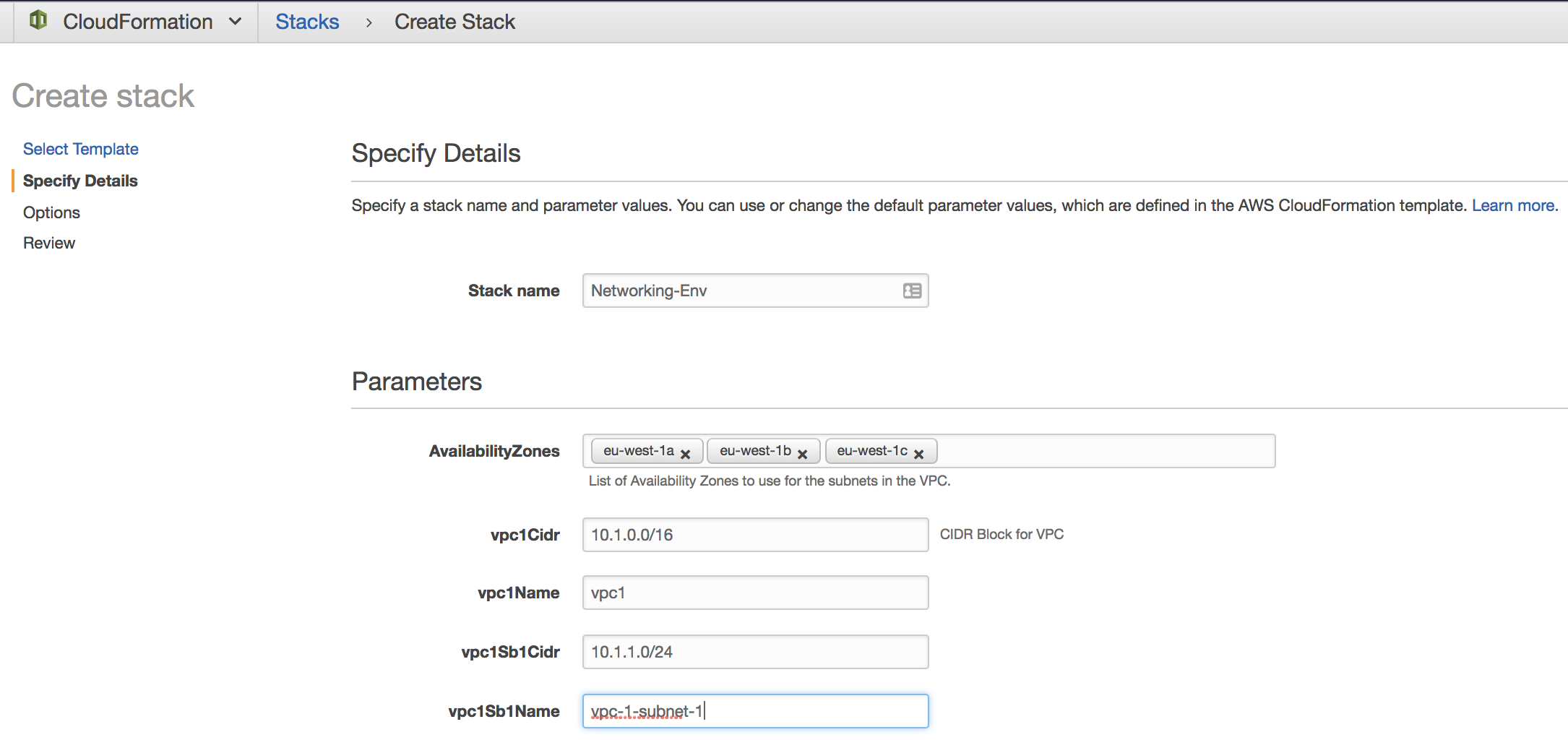
A stack can be easily created using the console - after clicking the ‘Create Stack’ button, you’ll be asked to specify the location of your template. You can specify a location in S3, or you can upload a template from your local machine. You’ll then be asked for a stack name and any parameter values that are needed for the template to run:
You’ll then have the option to review, after which you can create the stack.
You can also use the CLI to create the stack, for example:
In the above example, I called my stack “networking-environment” and am using a template named “net-env-master.json” to build it. I could have also passed in a parameters file using the –parameters switch on the command line.
Viewing Stack Information
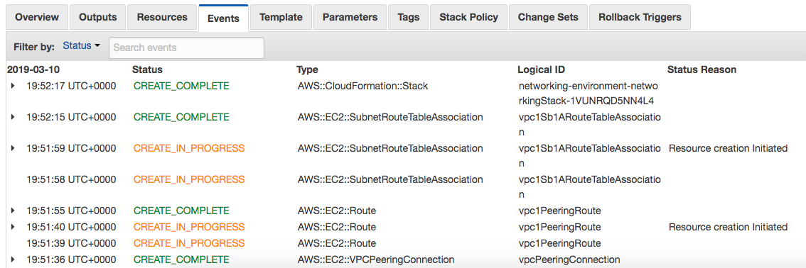
You can view information about the stack as it is being created, or after the stack creation process has completed. To start with, let’s look at events. In the CloudFormation console, if you check the box in the main area of the screen for the stack you’ve created, in the bottom half of the screen you’ll see another area where you can select “Events”. In this tab, you’ll see the status of each resource you are trying to create using CloudFormation - for example, CREATE_IN_PROGRESS, CREATE_COMPLETE or perhaps an error if the resource creation has been unsuccessful:
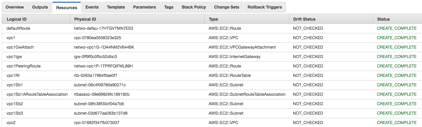
You can also see a list of all the resources created as part of the stack on the “Resources” tab:
One of the tabs in the bottom half of the page is named Outputs. An output from a CloudFormation stack is a piece of information related to that stack that you can use in other stacks by importing the info, or simply to view in the console so that you can use the information when configuring other parts of AWS. Here’s an example: let’s say you define an S3 bucket within a CloudFormation stack - because S3 buckets must have globally unique names, you use the template to generate a random name. However, you obviously don’t know what that random name will be, but you will need to use it for operations such as uploading or downloading data to / from that bucket. You can use outputs to show you that information once the stack has been created.
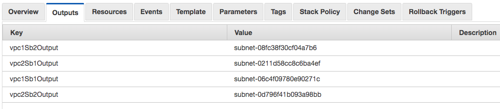
Here’s another example. In the following template, I need to get the subnet ID value for each of the subnets that I created through CloudFormation. I’m defining an output for four subnets (vpc1Sb1, vpc1Sb2, vpc2Sb1 and vpc2Sb2):
Once the stack has run, I can see the outputs and the corresponding values (the subnet IDs) in the CloudFormation console:
Change Sets
OK, so I have my Cloudformation template defined, I’ve created a stack and observed some of the outputs from it. Now though, I’ve decided that I need to make some changes to my template. Perhaps there are some parameters that I need to change; maybe the name of one of my instances is wrong and I need to alter it.
I could easily update my template to reflect the change and then simply rerun it, but it would be handy if I could view the changes and verify what impact they will have before I actually execute it. With Change Sets, you can do just that.
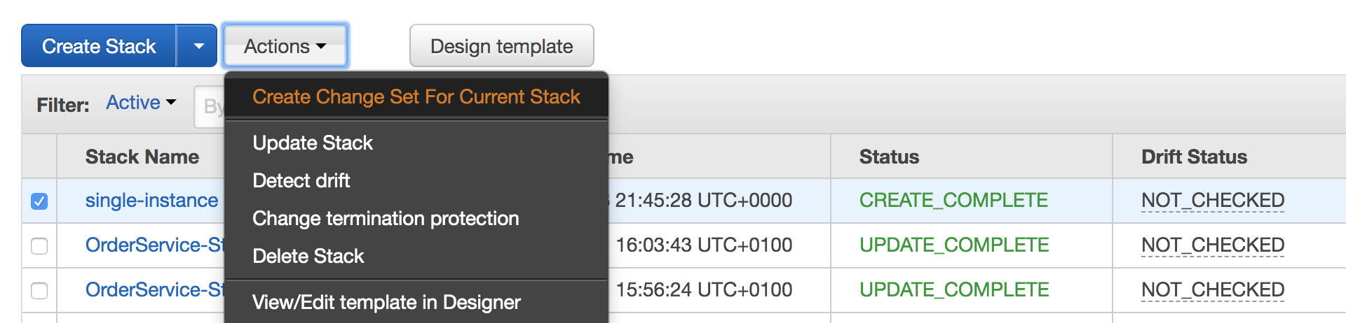
Here’s how it works: I have a Cloudformation stack named ‘single-instance’ deployed in my account - as the name implies, this template deploys a simple instance running Amazon Linux. I then decide that I want to make a change to the resource - specifically, I need to alter the size of the instance from t2.micro to m4.large. I make the change to the template and then create a new change set for the current stack:
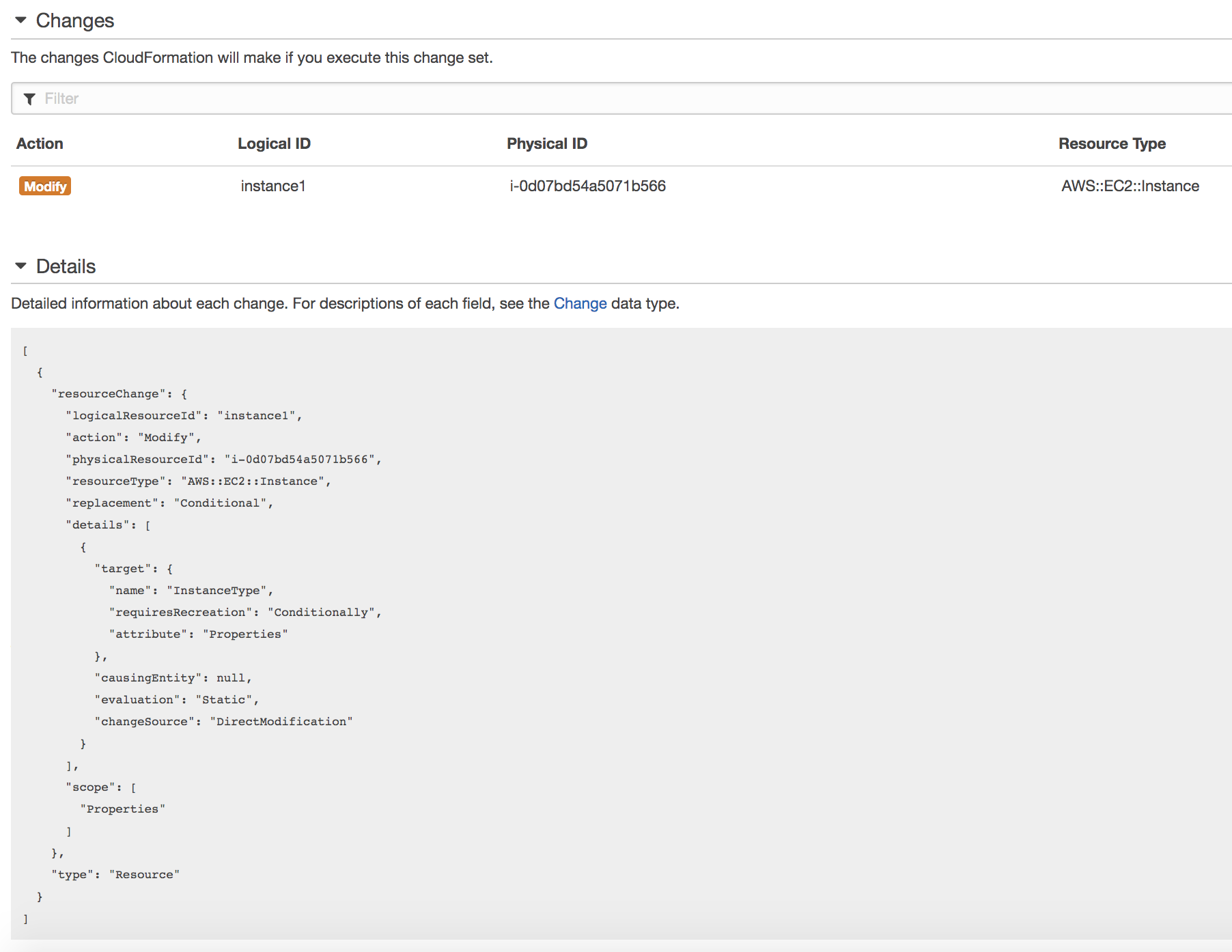
I’ll then be asked for the template (similar to when the stack was first created) - once this is done and I’ve given the change set a name, I’ll be able to view the details of the change in the console:
You can see in the details pane that the specific part of the template changing is the ‘InstanceType’.
I can then choose to execute the change set if the changes are acceptable, or delete the change set if I decide the changes aren’t what I want.
Drift Detection
One of the issues that some customers had in the past was how to manage the situation where a Cloudformation template was used to deploy resources, but then administrators were making changes directly to those resources rather than changing the template. There are lots of reasons why this might happen, for example a quick change is needed on a resource to fix a critical problem - the person making the change makes a note to go back and change the original template later so that everything is in sync, but never gets around to it. What I’ve described here is a scenario where the deployed stack has drifted from the original template. To alert you to this kind of problem, Drift Detection was introduced to Cloudformation.
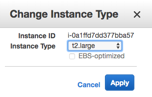
Drift Detection works by comparing the template used to deploy the stack to what the running stack actually looks like and can give you detailed information on the differences. Let’s look at an example. I’ve deployed the same ‘single-instance’ stack I used in the previous section to create single Amazon Linux t2.micro instance. After deployment though, the performance of this instance wasn’t where it needed to be, so I quickly went into the console and changed the instance type to t2.large:
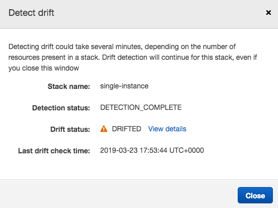
If I now go back to the Cloudformation console, select the stack and then choose ‘Drift Detection’ from the action menu, after a minute or so I’m told that there is indeed drift, with an option to view the details:
If I choose to view the details, I can see clearly the differences in the template (i.e. the instance size as t2.large vs t2.micro):
There’s a lot more to Cloudformation than I’ve been able to show you here - there is a huge amount of power and flexibility to allow you to automate the creation of resources inside AWS and we’ve only scratched the surface here. But hopefully this is enough to get you started :-)
Way back in part 3, I briefly discussed the AWS CLI as a way to interact with the AWS platform. In this post, I want to spend a bit more time looking at the CLI, as once you start to become more comfortable with AWS, it’s likely that you’ll find the console a bit limiting - mastering the CLI will ultimately make it easier and faster for you when using the platform.
Before I go any further, the first thing you need to do is actually install the CLI - the documentation explaining how to install the CLI on your local machine is available here. It’s easy to follow so I won’t duplicate it here.
Once you have the CLI installed, you’ll need to configure it with credentials to talk to your AWS account, as well as specifying the region to use. If you’re using your local machine with the CLI installed, have your access key ID and secret access key associated with your AWS account to hand. To configure credentials, run
aws configure
as follows:
aws configure
AWS Access Key ID [****************YGXQ]:
AWS Secret Access Key [****************IJy/]:
Default region name [eu-west-1]:
Default output format [None]:
Once you’ve configured this, you should be able to access your AWS account via the CLI. Note that the config and credentials are stored in a couple of files in the ‘~/.aws’ directory:
$ ls ~/.aws
config          credentials
If I take a look at my credentials file, I see the following (actual credentials removed!!):
What are the different sections for (default, eks-test-2, nocreds)? These are profiles that I have set up. Each of these profiles contains a different set of credentials (the ‘nocreds’ profile doesn’t contain any credentials at all due to some testing I was doing). To use these profiles, you can set an environment variable that specifies the profile - export AWS_DEFAULT_PROFILE=nocreds. Alternatively, you can specify the profile on each command that you run, for example:
8c8590cd6650:~ adaraffe$ aws s3 ls--profile=nocreds
An error occurred (AuthorizationHeaderMalformed) when calling the ListBuckets operation: The authorization header is malformed; a non-empty Access Key (AKID) must be provided in the credential.
As you can see, I’ve specified the ‘nocreds’ profile in the above S3 command, which - as you would expect - returns an error as that profile doesn’t contain any credentials.
As I mentioned in part 3, AWS CLI commands generally take the following form: firstly, the ‘aws’ command, followed by the name of the service you want to interact with (e.g. ec2, s3, etc) and then the specific action you want to take. Some examples are as follows:
aws s3 ls: lists all S3 buckets in your account
aws ec2 describe-instances: describes every EC2 instance in your account
aws ec2 start-instances –instance-ids i-079db50f95285d315: starts the instance with the instance ID specified
Changing the Output Format
By default, the AWS CLI outputs everything in JSON format. Using JSON as the output makes it easy to filter using the –query parameter (desrcibed in the next section) or using other tools such as jq. However, there might be times when you want more of a ‘human readable’ format, such as a table or just plain text.
Specifying –output=table after the CLI command returns the output as an ASCII table, for example:
You might find it easier to use the text output type if using Linux tools such as grep, sed, awk and so on.
Using –query to Filter Output
Taking the example in the section above - aws ec2 describe-instances, this potentially returns a lot of data, especially if you are running a lot of EC2 instances in your account. It’s highly likely that you are looking for more specific information - for example, you might be looking for the private IP address associated with one specific instance. Fortunately, this is easy to achieve through the use of CLI queries.
Query strings use the JMESpath query specification. To demonstrate how it works, let’s look at some examples.
Firstly, let’s say I want to find out what the instance type is for each of my EC2 instances. I can get this information using the following command:
Let’s look at how that query works. Firstly, the ‘Reservations[].Instances[]’ causes the query to iterate over all the instances in the list. The second half of the query (‘[InstanceId,InstanceType]’) then returns only the two elements (InstanceID and InstanceType) from each instance. Finally, I specified that I wanted the output to be in table format. I can make the table even more friendly:
This time, I tweaked the command so that the table would have the headings ‘Instance’ and ‘Type’ to make it a bit more readable. Here’s another example - what if I wanted to find the private IP address of a specific instance? Here’s how I could do it:
aws ec2 describe-instances --query'Reservations[*].Instances[?InstanceId==`i-0f77eeba0d2835444`].[PrivateIpAddress]'--output text
172.31.27.82
In this example, I’ve searched for a specific instance ID in the first half of the query (using ?InstanceId==i-0f77eeba0d2835444) and then in the second half of the query I’ve asked for only the ‘PrivateIpAddress’ element to be returned.
Generating a CLI Skeleton
The AWS CLI has the ability to accept input from a file containing all of the parameters required, using the option –cli-input-json. However, it can be difficult to know which parameters you need and what they are called. To help with that, the CLI provides a way to generate a ‘skeleton’ set of parameters for a given command, which then allows you to fill it in and use it as input via the –cli-input-json option.
Here’s an example: I want to create a new VPC using the CLI - to generate the CLI skeleton, I can do the following:
Now, all I have to do is create a file containing the information in the skeleton with the values filled in (and with ‘DryRun’ set to false), and then refer to that file in the command:
In part 5, I talked briefly about the disk options available to you when running EC2 instances - you have the choice of using instance store based disks (i.e. a disk that is directly attached to the underlying host machine that your instance runs on), or to use an Elastic Block Store (EBS) based volume.
Instance store disks are fine for temporary data storage, but aren’t a great choice for data that you want to be persistent - if the underlying host were to fail, or you happen to stop or terminate your instance, the data you have stored on the instance store based disk will be lost forever. If the thought of that upsets you, EBS based disks are the way to go.
One of the key points about EBS is that a storage volume is not “tied” to a particular instance - it’s entirely possible to attach EBS volumes to any instance, as long as that instance sits in the same Availability Zone as the volume. So in other words, I could detach an EBS volume from an instance, destroy that instance and then re-attach the EBS volume to a new instance that I create later.
EBS provides a number of different types of storage volume that differ in terms of both performance and cost. Let’s take a look at what’s on offer.
EBS Volume Types
The volume types on offer from EBS fall into two main categories:
SSD backed volumes: As the name implies, these volumes are all based on solid state drives and are the recommended option for many workload types.
HDD backed volumes: Volumes based on hard disk drives (i.e. spinning disks) are recommended for throughput intensive workloads.
Amazon then breaks these categories down further into the following volume types:
General Purpose SSD (also known as ‘gp2’): This is a good choice for the majority of applications - it provides good level of performance, albeit potentially less ‘consistent’ than the io1 volume type (covered next). The key thing with gp2 volumes is that they provide a certain number of IOPS (I/O Operations per Second) based on the size of the disk. You don’t specify the number of IOPS directly, but instead get a certain level of ‘base performance’ depending on how large the disk is. You also get a certain amount of burst capacity based on a credit system - burst credits are replenished regularly and are consumed whenever you need more than the baseline performance. But of course, if you use up your credits, you are back down to the baseline performance level.
Provisioned IOPS SSD (also known as ‘io1’): The difference between gp2 and io1 is that with io1, you are specifying a certain number of IOPS and the system will deliver it - there is no burst credit system as there is with gp2, therefore the number of IOPS you receive is potentially more consistent. As a result, io1 volumes tend to be used for workloads requiring higher IOPS or critical apps that require the more consistent performance.
Throughput Optimised HDD (also known as ‘st1’): The first of the HDD offerings provides a relatively low cost volume type with decent throughput. This kind of vlume tends to be useful for big data workloads, log processing, or data warehouses. One thing to bear in mind with HDD volume types is that you cannot use them as boot volumes for EC2 instances.
Cold HDD (also known as ‘sc1’): The sc1 volume type offers the lowest cost storage available within EBS. It is typically designed for data that isn’t all that frequently accessed, although still offers a reasonable level of throughput.
Note also that there is a fifth type of volume called Magnetic (also known as ‘standard’) which is still available today, although this is considered to be part of the ‘previous generation’ of storage and generally speaking, shouldn’t be used for new apps.
Creating EBS Volumes
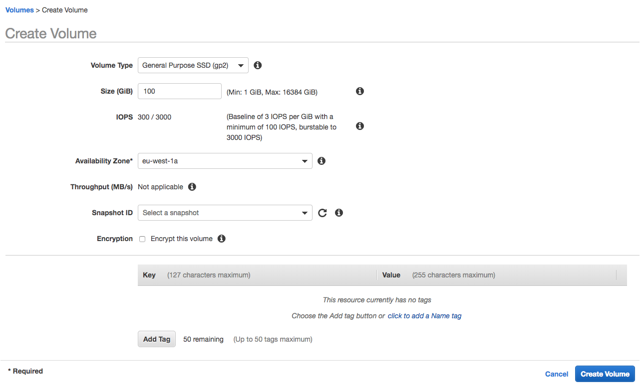
Creating an EBS volume is a pretty easy process. Accessed from the EC2 part of the AWS console, you specify the volume type (as discussed above), the number of provisioned IOPS (in the case of the io1 type), how large you want your volume to be, whether you want your volume to be created from a snapshot (discussed in the next section below) and also whether the volume should be encrypted. Here’s an example:
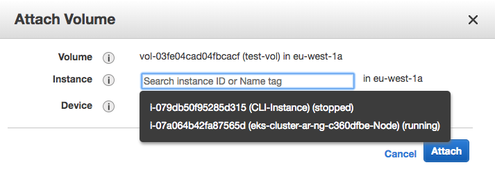
You can then attach the instance to an EC2 instance that resides in the same Availability Zone by selecting the volume and then using the ‘actions’ menu:
Of course, an easier way is to just create the volume as part of the EC2 instance creation, in which case you don’t need to worry about attaching it - that just happens automatically as part of the instance creation.
You can also use the AWS CLI to create volumes - for example:
Now that we know how to create an EBS volume and use it from an EC2 instance, let’s look at how we can back up our volumes using Snapshots.
Snapshots
An EBS snapshot is simply a point-in-time back up of the data blocks on an EBS volume. When you take an initial snapshot from an EBS volume, all blocks are copied from the volume to the snapshot - pretty straightforward. However, if you then decide to take subsequent snapshots from the same volume, only the data that has changed since the last snapshot are copied over. This is significant, because it means that a) data is not duplicated many times, which saves and storage costs and b) the time is takes to create the snapshots is greatly reduced.
How does this actually work in practice? What actually happens is that when changed or new data is copied, a new snapshot is created and linked to the previous snapshot. You can read more about this process here.
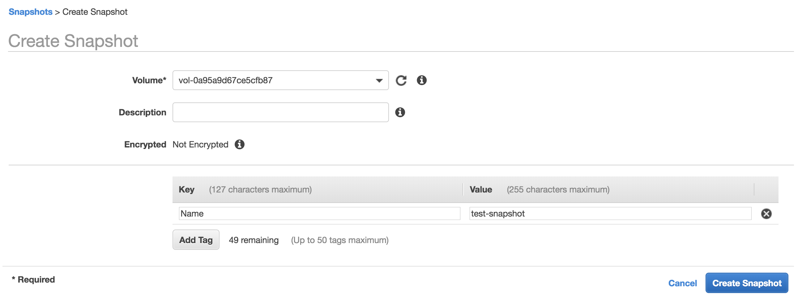
Let’s look at how you create a snapshot. From the left hand menu within the EC2 part of the console, select ‘Snapshots’ and then ‘Create Snapshot’. You’ll then see the following screen:
As you can see, this is very simple - you need to specify the volume that the snapshot will be taken from and optionally provide a description and tag. Now once you press the ‘Create’ button, you’ll see a state of ‘Pending’ under the snapshot item that results - what is actually happening here is that the data from the volume is being copied to the snapshot in the background. Depending on how large the volume is, that might take a few hours. Where is the data actually being stored? The snapshots themselves are all stored in S3.
OK, so now that we have our snapshot, what can we do with it? Several things are possible:
We could create a new EBS volume from the snapshot.
The snapshot can be copied, including to other regions. You might want to do this for a number of reasons, including migrating instances to a different region, disaster recovery purposes, expanding to other geographies, etc.
A new AMI (Amazon Machine Image) could be created from the snapshot for use when creating new EC2 instances.
We can also share the snapshot with other AWS accounts.
All of the above actions can be carried out from the ‘Actions’ menu within the snapshots area.
I mentioned at the beginning of this section that snapshots can be used to backup up EBS volumes. However, it’s important to understand that snapshots are block level backups - they are not file level backups. What that means is that you can’t simply dip into a snapshot and pick individual files out of it, for example if you have deleted something you shouldn’t have. In order to ‘get at’ the data within the snapshot, you’ll need to do the following:
Create a new volume from the snapshot.
Attach the new volume to an EC2 instance and mount it.
Access the files through the EC2 instance.
Automating EBS Snapshots
For snapshots to be useful as a backup mechanism, there needs to be some way of scheduling snapshot creation automatically - it’s no use if you have to create a new snapshot manually every day. Fortunately there is a way to do this, using a feature called Data Lifecycle Manager (DLM).
DLM can be accessed from the left hand menu of the EC2 area of the console. The primary method for identifying which volumes to back up is by using tags - for example, I could tag each of my volumes with a particular tag (say ‘snapshot:target’) and then configure DLM to look for all volumes with that particular tag and back them up.
In the following example, I want to back up all EBS volumes in my Kubernetes cluster, therefore I am configuring DLM to target all EBS volumes with a tag of ‘EKS-Cluster-1’:
I then tell DLM how often to create the snapshots (every 12 or 24 hours) and the time I want the snapshot start time to be.
OK, hopefully that gives you enough information about EBS to get going. See you next time!
The Simple Storage Service (usually referred to as S3) was one of the earliest - and one of the best known - services available from AWS. But what exactly is it and what does it provide? At the most basic level, S3 provides users with the ability to store objects in the cloud and access them from anywhere in the world using a URL. What do I mean by ‘objects’? An object can be pretty much anything you like - files, images, videos, documents and so on. One of the defining characteristics of S3 is that for all practical purposes, it provides an unlimited amount of storage space in the cloud. Users of S3 pay only for the storage they use on a per Gb basis. There are also charges to retrieve data - these charges vary depending on which tier of storage you are using.
Whereas S3 is designed for every day storage purposes, S3 Glacier(recently renamed from ‘Glacier’) is designed for long term storage and archival and is priced with this in mind (i.e. it is cheaper to store data). However, the trade-off is that retrieving data from S3 Glacier can take longer than with regular S3 storage, plus it is typically more expensive to perform those retrieval operations.
Durability of Data
Data durability refers to how likely it is that data will be subject to corruption or loss. AWS state that the S3 Standard, S3 Standard-IA and S3 Glacier tiers are designed for 99.999999999% durability. What that works out to is that if you store 10,000,000 objects in S3, you could expect to lose a single object once every 10,000 years. So, there’s still a chance, but I wouldn’t be losing any sleep over it.
How do AWS achieve these levels of durability? A major factor is that data is stored on multiple devices across availability zones. So if I write an object to S3, that data is stored redundantly across multiple AZs (normally three) and a SUCCESS message is only returned once this has been done. There are other mechanisms in place to detect data corruption, such as MD5 checksums and CRC checks - all of this adds up to an extremely reliable system.
S3 Storage Tiers
To provide the maximum amount of flexibility, AWS provides a number of storage tiers, each with differences in pricing and capabilities (such as retrieval times). I’ll cover the tiers available at the time of writing, but be aware that AWS do occasionally add new storage tiers, so it’s worth checking the AWS documentation.
Firstly, there is the S3 Standard tier. This is the ‘original’ S3 storage tier and is widely used for ‘general purpose’ storage. It is highly available (99.99% over a year) and resilient and tends to be the ‘default’ option when users need frequent access to their data.
Secondly, there is the S3 Standard - Infrequent Access (S3 Standard-IA) tier. This tier is similar in many ways to the S3 Standard tier, however the main difference is that it is designed for data that needs to be less frequently accessed, therefore the per Gb storage costs are cheaper. However the trade-off is that it costs slightly more to retrieve that data. S3 Standard-IA is also designed for a slightly lower availability (99.9%) compared to S3 Standard.
Next up is S3 Standard - One Zone Infrequent Access (S3 Standard-One Zone-IA). As you can probably guess from the name, the primary difference with this tier is that data is not copied across three availability zones as is the case with the previous two tiers we discussed. Because of that, availability drops slightly (to 99.5%), plus there is a very small risk that data could be lost in the event of an availability zone being destroyed.
A more recent addition to the family is S3 - Intelligent Tiering. The idea behind this tier is that AWS will automatically move data between tiers on your behalf, with the goal of ensuring that your data is always kept in the most appropriate tier, cost wise. For example, if S3 notices that some data hasn’t been accessed for 30 days, it will automatically move that data into the Infrequent Access tier. If that data is accessed, S3 will move it back into the S3 Standard (frequent access) tier.
S3 Glacier is the ‘original’ Glacier service, now brought into the main S3 family and designed for archiving of data. Glacier provides very cheap storage and different options for data retrieval, depending on how quickly you need to get that data back (costs differ accordingly).
Announced at re:Invent 2018, S3 Glacier Deep Archive will provide the lowest cost storage option available from AWS - this tier is designed for data that needs to be retained on a longer term basis (for example, 10 years or longer). It offers an alternative to tape based storage systems, with retrieval times of up to 12 hours.
Now that we’ve seen the different storage tiers available, let’s dive in and start to look at how S3 actually works.
S3 Buckets
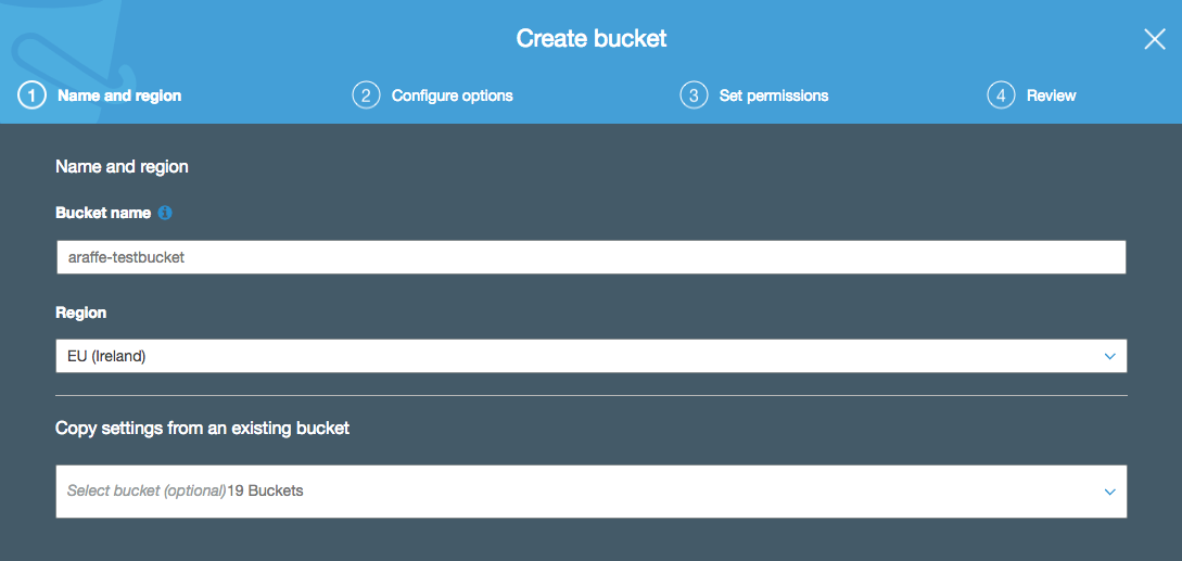
Before you can store anything in S3, you need to create a bucket. A bucket is really nothing more than a folder that will be used to hold your storage objects - it is a place for you to store your own objects in the cloud, and which no-one else can gain access to (unless you grant access). You can create a bucket easily using the S3 API, CLI or AWS console:
Notice in the above screenshot that I’m being asked for a bucket name - in this example, I’m calling it ‘araffe-testbucket’. I could have tried calling it simply ‘testbucket’, but that probably wouldn’t have worked - the reason for that is that S3 bucket names must be globally unique. By globally unique, I don’t just mean they need to be unique within your account - they have to be unique everywhere (i.e. the whole world). So if another user of S3 has taken the bucket name ‘testbucket’ (quite likely), I won’t be able to use it. It’s probably unlikely that someone else has used ‘araffe-testbucket’ though, so I should be safe with that one.
If you’re more a fan of the command line, you can create a bucket using the following syntax:
aws s3 mb s3://araffe-testbucket
There are a number of other options you can configure while creating your bucket, some of which I’ll cover later. However, there is one important configuration item we should deal with now - public access to buckets.
Public Bucket Access
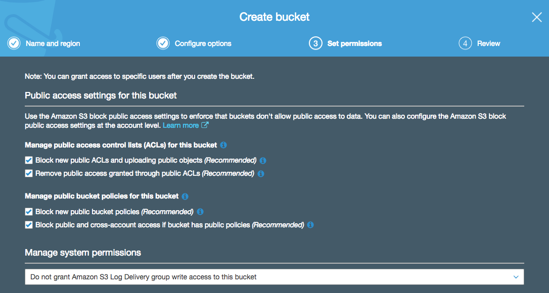
If you follow the bucket creation config pages all the way through, eventually you’ll be presented with a page that asks you to consider the public access settings for your bucket:
What this page is actually asking you is: “Do you want to prevent anyone from applying a policy that will make your bucket open to the public? Or would you prefer to untick these boxes and potentially allow access into your bucket from the entire universe?”. Public access to your bucket is exactly how it sounds - the ability for anyone in the world to access objects inside your S3 bucket. OK, there are a few use cases for this, but in general this is something you probably want to avoid doing.
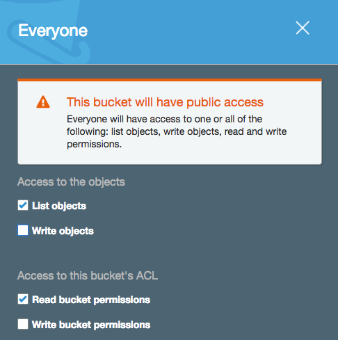
If I untick the boxes in this dialog box and then go on to alter the permissions for my bucket to make it public, I’m presented with a large warning banner informing me of my potential stupidity:
So, you can’t say you weren’t warned :-).
Bucket Policies
In the Identity and Access Management (IAM) post, I mentioned that there were two types of policy - identity based and resource based (where a policy is applied directly to a resource rather than a principal). An S3 bucket policy is one example of a resource based policy and allows you to grant access to your S3 resources.
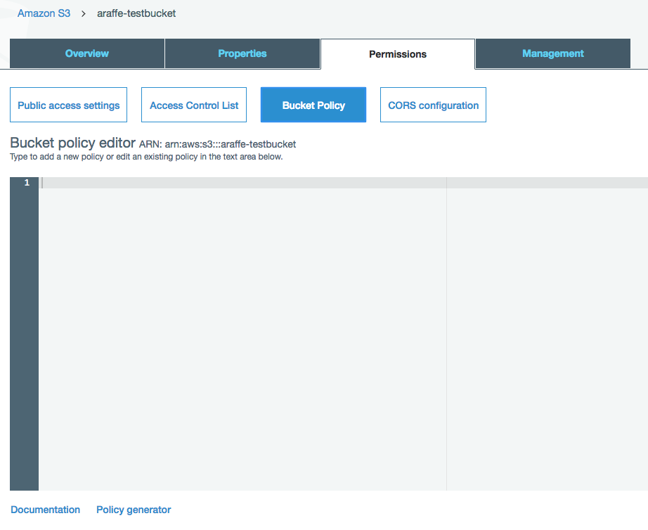
Let’s start with a simple example. Say I want to allow read access into a specific S3 bucket from anyone (i.e. anonymous access). As I mentioned earlier, allowing public access to your S3 buckets isn’t generally the best of ideas, but there might occasionally be reasons for doing so (running a static website on S3 and therefore needing people to access objects). Going back to the bucket I created earlier, if I click on it in the console and then on ‘permissions’, I see ‘Bucket Policy’ in the list of options I have:
OK, so now I have a ‘bucket policy editor’ - what do I put into that? Well, the language is actually the same as we saw earlier in the IAM post, using resources, actions, effects and so on. So if I want a policy that allows anonymous access to my bucket, I could use a policy as follows:
Note that in order to apply this policy, I would first have to untick the option that blocks public access in the ‘public access settings’ dialog that we discussed in the section above.
Here’s another example: imagine I want to allow access into my S3 bucket only from a certain range of IP addresses. Here’s how the policy might look:
You might be thinking to yourself that the idea of writing these policies out by hand is a bit daunting - if that’s the case then have no fear, because at the bottom of the bucket policy editor screen (shown above), there is a link to a policy generator. This will guide you through the process of defining your policy using drop down boxes and then present you with the policy document at the end, which you can simply cut and paste into the bucket policy editor.
Uploading and Download Data from S3
OK, so you’ve created an S3 bucket. That’s very nice, but not all that useful unless you can actually get some data into that bucket and download it when you need to.
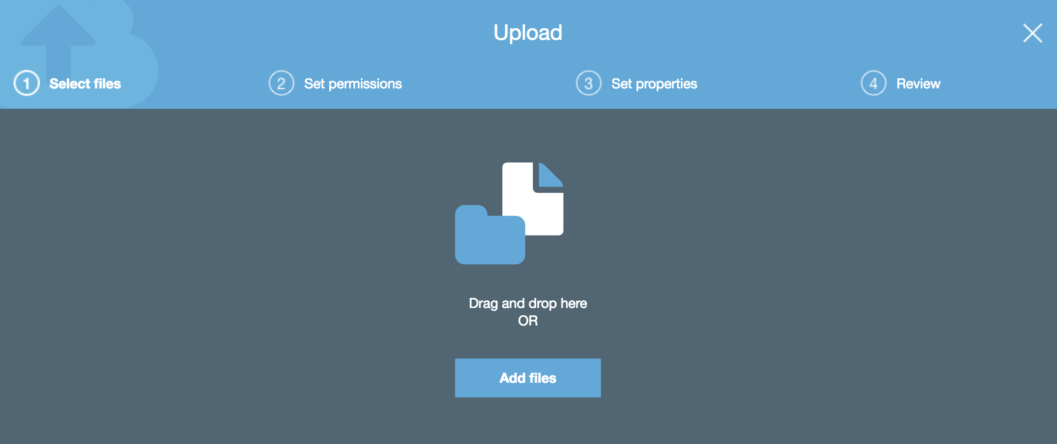
Uploading an object to S3 using the AWS management console is one of the simplest operations you can do - you simply click on the bucket that you have created and then click on ‘Upload’. From here, you can drag and drop or select files from your local computer:
Once you’ve chosen the files you want to upload, you can set permissions on them and choose which storage tier (Standard, Standard-IA, etc) the objects will use.
To download objects using a browser, you can get the URL for any given object by checking the box next to it in the S3 management console - a box will open on the right hand side of the screen showing information about the object, including the URL for the object. If the person using the URL has permission, they will be able to download that object.
Using the aws s3 cp Command
If you aren’t a fan of graphical interfaces and would rather use a CLI based tool to move your data around, you can use the AWS CLI to copy data instead.
The ‘aws s3 cp’ command is very flexible and allows you to perform all sorts of operations, including setting permissions, managing encryption, setting expiry times and more. Let’s look a couple of simple examples to get started:
Firstly, you can use the aws s3 cp command to copy a single file from your local machine to your S3 bucket - in this case, I am copying a file named ‘hello.txt’ from my laptop up to my ‘araffe-testbucket’ bucket in S3:
aws s3 cp hello.txt s3://araffe-testbucket/hello.txt
upload: ./hello.txt to s3://araffe-testbucket/hello.txt
You can see that the operation has succeeded by the output after the command has executed (you can also check using the management console of course).
I can also copy the file back from S3 to my local machine:
aws s3 cp s3://araffe-testbucket/hello.txt hello.txt
download: s3://araffe-testbucket/hello.txt to ./hello.txt
What if I want to copy a large volume of files and directories to S3 at once? I can use the ‘–recursive’ switch to copy a complete directory structure, for example if I want to copy the directory ‘Adam’ with all subdirectories:
aws s3 cp Adam s3://araffe-testbucket/ --recursive
These are just simple examples - it’s worth checking out the documentation for full details on what you can do with the S3 command line.
Using Pre-Signed URLs
When you upload objects to S3, those objects are private, unless you have configured that to not be the case (which isn’t normally advisable). However, there will be times when you want to make objects available on an exception basis but still keep them private overall. Is that possible? It is, using pre-signed URLs.
A pre-signed URL is a special URL that you create with your own credentials that gives anyone with the URL access to the object in question, on a time-limited basis. Let’s say I want to give someone access to the ‘hello.txt’ file that I uploaded in the last section. To do that, I can use the following CLI command to generate a pre-signed URL for this object:
aws s3 presign s3://araffe-testbucket/hello.txt
This command generates a URL that you can give to the person who needs access to your file - note that by default, this URL expires in 3600 seconds, although you can configure this expiration using the ‘–expires-in’ switch.
S3 Versioning
I have an S3 bucket which I’m using to store a whole bunch of files in. One day, I make a change to one of my files and then re-upload it to my S3 bucket, overwriting the old one. Then - to my horror - I realise that I’ve made a terrible mistake with the updated file and need to go back to the old one. Unfortunately I’ve already overwritten both my local copy and the one in S3, so I’m now in big trouble. If only there was a way to prevent this from happening…
Versioning in S3 allows you to keep multiple versions of the same object within a single S3 bucket. What that means in practice is that you can overwrite an object (like I did in my example), however the object will be created with a new version number, while the old version will remain in place. If I make a mistake, I can restore the previous version of the object and all will be fine with the world. Let’s see how this works.
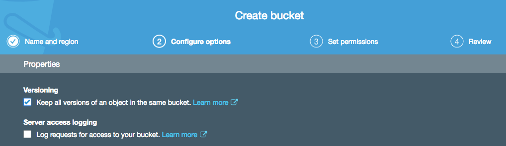
I’m once again creating an S3 bucket, but this time I am enabling versioning on that bucket (note that you can also enable versioning on previously created buckets):
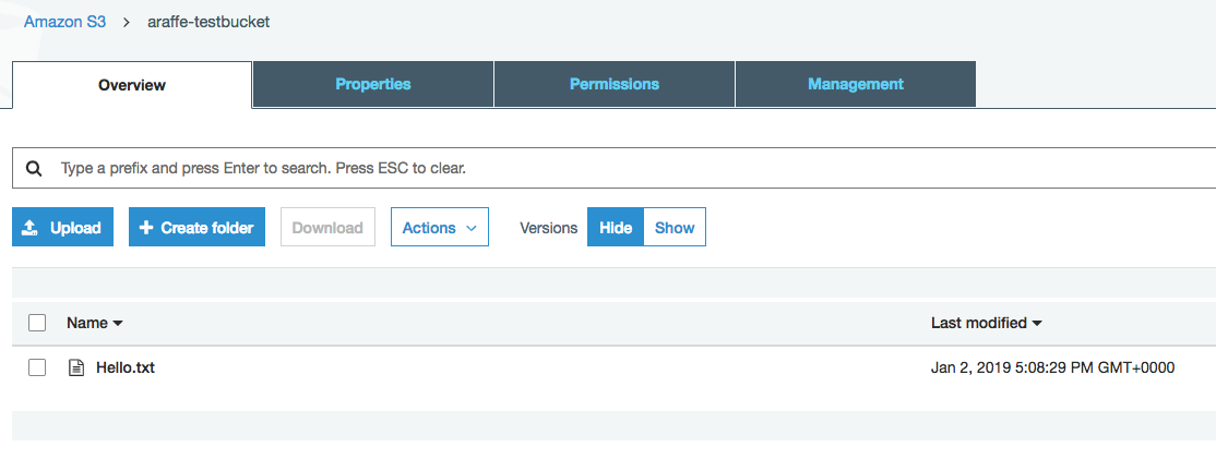
I then upload a file into my new bucket called ‘hello.txt’:
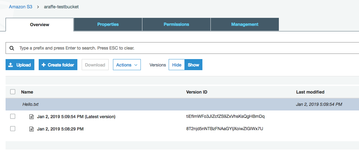
I now make an update to my text file and re-upload it to my bucket. Once I have done this, because versioning is enabled on the bucket, I can see both versions of the file:
I can easily download either of the versions using the normal methods. If I want to, I can delete the latest version of the file, which will result in the older file being left in the bucket and still available for download.
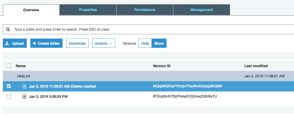
Versioning also affects how objects behave when they are deleted. Deleting an object in a versioning enabled bucket doesn’t actually delete the object at all - instead, a ‘delete marker’ for that object is placed in the bucket. You can see this in the screenshot below, after I have deleted the file ‘hello.txt’:
OK, but what if I want to recover my file? Simple: I just remove the delete marker - this restores the original object to the bucket.
One thing to bear in mind when using versioning is the impact it may have on costs. As you are now potentially storing multiple versions of an object in your bucket, these are charged at the normal rates for the tier you are using.
Finally, once versioning is enabled on a bucket, it cannot be disabled - only suspended. Suspending versioning on a bucket means that no new versions of objects will be created, however any existing object versions will be kept.
Lifecycle Management
At the beginning of this post, we discussed the various storage tiers available in S3 (Standard, Standard-IA, Standard-One Zone-IA, and so on). It’s of course perfectly fine in many cases to stick all of your objects into the Standard tier and be done - equally however, you may find that this isn’t the most cost effective strategy for storing your objects and that it’s better to store some objects in the ‘lower’ tiers. The problem is, how do you manage this if you have a huge amount of objects stored in S3? It’s not really feasible to manually move objects around between tiers. This is where the lifecycle management capabilities of S3 come in.
Lifecycle management allows you to specify a set of rules that state that objects are either moved between S3 tiers when certain conditions are met, or that the objects are deleted after reaching a particular expiration time. As an example, you might upload a set of documents that are accessed frequently for the first month, after which they are hardly ever accessed and therefore better suited to one of the infrequent access tiers.
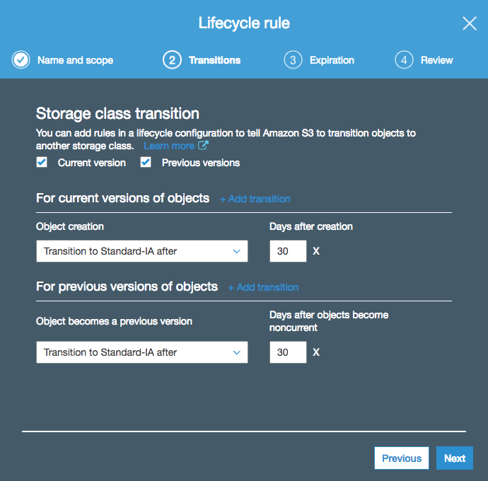
Here’s an example: in the screenshot below, I am creating a lifecycle rule that transitions both current and previous versions of my objects (I have versioning enabled on my bucket) to the Standard-IA tier after 30 days (this is actually the minimum amount of days I can configure for the Standard-IA tier):
On the next page, I am configuring an expiration of 90 days for my objects, including permanent deletion of previous versions:
I could have selected any of the other storage tiers, such as intelligent tiering or S3 Glacier if I wanted to archive my objects after a certain amount of time.
S3 also has a storage class analytics tool which looks at the storage access patterns for your bucket and helps you to decide which lifecycle policies you should configure, which storage class to transition to and so on.
Cross-Region Replication
Under normal circumstances, any objects that you upload to an S3 bucket will stay within the region where that bucket was created - there are obvious reasons for this relating to compliance, etc. You certainly don’t want data to be moved into other regions without your knowledge.
However, there are some situations where you might actually want your data to be copied to another region. For example, where customers reside in multiple geographic locations, you might want to maintain copies of data in two AWS regions that are geographically close to those customers. There might also be legitimate reasons relating to disaster recovery. To support these use cases, AWS provides the ability to perform cross-region replication of objects in S3.
Cross-region replication works exactly as it sounds - any objects uploaded to an S3 bucket after enabling cross-region replication are copied asynchronously to a bucket in another region of your choice. There are a couple of things to bear in mind when enabling cross-region replication:
Only objects that you upload after enabling cross-region replication are copied. Any objects that existed before you enabled the feature are not replicated.
By default, objects will be replicated using the same S3 storage class as the source object uses. So if your source object is stored in S3 Standard-IA (infrequent access), the replicated object will also be stored in the Standard-IA storage class. You can however specify a different storage class for the replicas should you wish.
You can replicate objects between S3 buckets in different AWS accounts.
You can replicate encrypted objects, although this is not the default - you have to tell S3 to do it.
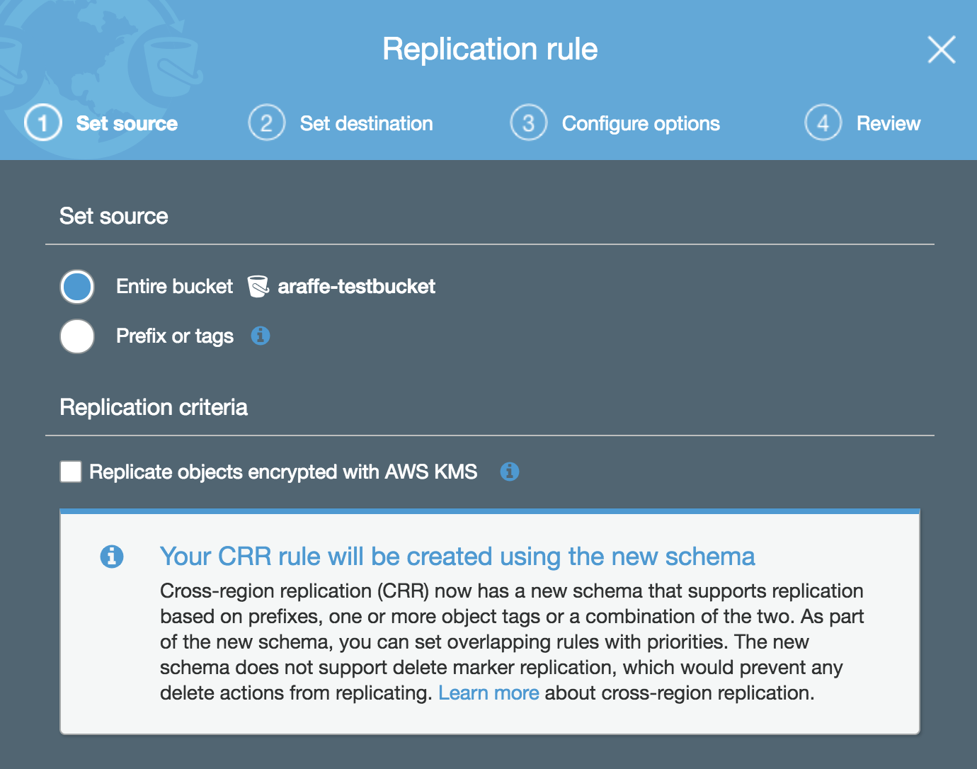
Let’s have a look at how this is configured. From the ‘Management’ tab within the S3 bucket, click on ‘Replication’ and the following dialog appears asking you set the source:
Note here that you can choose to replicate objects in the entire bucket, or you can replicate only objects with a particular tag or prefix (for example, any objects that have a name beginning with ‘photos’).
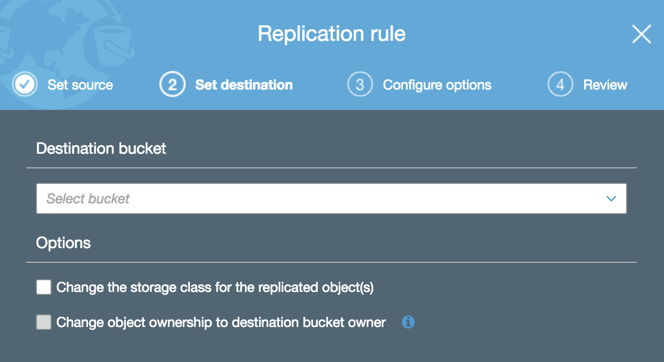
You’re then asked to specify the destination bucket. At this point, you can also change the storage class for replicated objects as well as alter the object ownership:
Note that for cross-region replication to work, you must have versioning enabled (see section above).
Encryption
S3 provides the ability to encrypt the data residing in your buckets at rest. What does ‘at rest’ mean? It is simply the ability to encrypt the data while it resides on disks inside a data centre. The opposite of ‘at rest’ is ‘in transit’, where data is encrypted as it is transmitted from place to place.
As a general rule, you should always choose to encrypt data at rest when you use S3 - there isn’t really a reason not to. When you create the bucket, there is an option to automatically encrypt objects when you upload them to S3 - you should check this box :-) When enabling encryption, you have a number of choices around how the encryption keys are managed:
The first option you have is to use Server-side encryption with S3 managed keys (SSE-S3). Choosing this option essentially means that S3 manages the encryption keys for you - you don’t have to worry about any aspect of key management. You simply upload your objects to S3 and each object is encrypted using a unique key.
Alternatively, you could go with Server-side encryption with KMS managed keys (SSE-KMS). KMS stands for Key Management Service - this is a service provided by AWS that allows you to create and manage encryption keys. So if you choose this option, your encryption keys will be managed within KMS, rather than directly within S3. What’s the difference? With KMS managed keys, you get some additional benefits over and above SSE-S3, such as the ability to create and manage the encryption keys yourself, as well as audit trails for the master key.
Finally, you could choose Server-side encryption with customer managed keys (SSE-C). With this option, you are responsible for managing the encryption keys yourself - Amazon does not store any encryption keys. Instead, you pass the encryption key with the request and S3 uses that to encrypt or decrypt the data. Of course, as Amazon isn’t storing your encryption keys, you need to be careful not to lose them - if you do, you’ve lost your data!
There is one more option not mentioned in the above list - you can of course encrypt the data yourself before you send it to S3. You can do that using either KMS managed keys or keys that you manage yourself - the key point is that S3 is not encrypting or decrypting anything as that is happening on the client side.
That just about rounds things out for S3. There’s more to learn but this post covered the basics and should give you enough info to get going. Thanks for reading!
Networking is an important topic in AWS. Many of the networking concepts in AWS are somewhat similar to what you might find in traditional, on-premises networks - IP addresses, subnets and routing tables don’t just disappear in the cloud! However, there are some differences as well, which I’ll try and cover in this post. Let’s jump in, starting with the most fundamental building block used in AWS networking: Virtual Private Clouds.
Virtual Private Clouds (VPCs)
A Virtual Private Cloud (VPC) is a private, isolated network within the AWS cloud. Within a VPC, you can run the services that you need, including EC2 instances, RDS instances, container clusters and a host of others. The key here is that VPCs are completely dedicated to you - there is no ‘sharing’ of VPCs with other customers or entities (unless you specifically want that to happen), which means you can be safe in the knowledge that services running inside your VPC are isolated from anything else on the AWS cloud, if that is your goal.
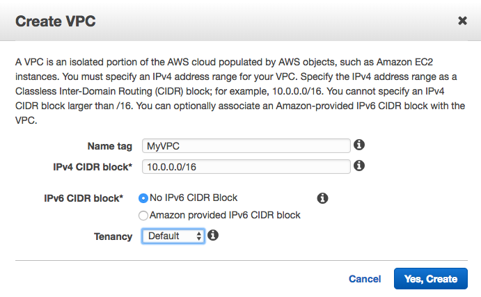
Creating a VPC is easy - you need to name it and give it an IP address space (CIDR block):
In fact, you don’t even need to create a VPC yourself if you just want to deploy a few services quickly and easily - AWS helps you out by providing a default VPC with every account. This default VPC has a couple of settings that custom VPCs do not - specifically, any instances launched within the default VPC will have a public IP address automatically assigned and will have Internet access directly from that VPC. Custom VPCs do not have this behaviour by default, although it can be easily changed. More on public IPs and Internet Gateways later. The default VPC is configured with a CIDR block of 172.31.0.0/16 and has 3 subnets configured, one per AZ. Each of these subnets has a /20 IP range. Speaking of subnets…
Subnets
To deploy services into a VPC, you are going to need at least one subnet. Each subnet has a specific IP address range (taken from the main VPC CIDR block), so for example, the default VPC (as mentioned above) has a CIDR block of 172.31.0.0/16, with the first subnet using 172.31.0.0/20, the second subnet using 172.31.16.0/20 and so on. Obviously if you decide to create your own VPC, then you can address this as you like.
Now here’s an interesting thing about subnets: they are directly associated with Availability Zones (AZs). When you create a subnet, you need to choose which AZ that subnet is associated with (or you can let the AWS platform choose for you if you don’t care too much). So, with a single VPC and two subnets, our topology might look something like this:
It’s important to understand that a subnet cannot span AZs - it always sits entirely within a single AZ.
Public and Private Subnets
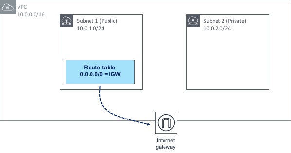
A subnet can be configured either as public or private within the AWS cloud - in other words, it can allow direct access to the Internet, or it can remain inaccessible to the outside world, unless you have another means of getting to it (via a Direct Connect link or VPN connection for example). But what do we actually configure to cause a subnet to be either public or private? It comes down to a combination of a couple of things: an Internet Gateway (IGW) and accompanying route table that routes traffic through that IGW. This is best explained with a diagram:
Let’s look first at the Internet Gateway. The IGW is deployed and attached to the VPC itself - not to any particular subnet. However, any subnet has the ability to route through that IGW, which is exactly what Subnet 1 is doing. A route table has been created and attached to Subnet 1. Within that route table, there is a route towards 0.0.0.0/0 (this is known as a default route, as it essentially means “any traffic that doesn’t match any other routes should use this one”). The default route in this case points to the IGW as a next hop - this causes any traffic destined for the Internet to take the path towards the IGW, which is what makes Subnet 1 a “public” subnet.
Now if you look at Subnet 2, there is no such route table pointing towards the IGW, which means there is no possible path that traffic can take out to the Internet - in other words, Subnet 2 is considered “private”.
But simply making a subnet public doesn’t necessarily mean that traffic from its associated instances can automatically reach the Internet - for that to happen, we also need to consider the IP addressing within the subnet.
Public IP Addresses
When you create an EC2 instance and attach it to a subnet & VPC, that instance will automatically receive a private IP address to allow it to communicate with other instances and services internally (or even to on-premises environments via a Direct Connect link or VPN connection). However, a public IP address will allow the instance to communicate out to - and be accessible from - the Internet.
There are two types of public IP address. The first is a dynamically assigned public IP - this type of address is assigned to an instance from Amazon’s pool of public IPs. That address is not “owned” by you and it isn’t associated with your account - think of it as if you are “borrowing” the address from AWS.
Now, there’s an important point to remember about public IP addresses: if you either stop or terminate the instance, the public IP address that is attached to that instance is released back into the pool. What that means in practice is that if you restart the instance, you are extremely unlikely to end up with the same public IP address you had previously. Is that an issue? Maybe, maybe not. In many cases, having a public IP address that could change won’t be a problem (e.g. if you are relying on DNS resolution), but what about if an application is hard coded to use a specific IP address, or if there is some kind of firewall rule in place that allows only a specific IP? In that case, you might want to look at Elastic IPs instead.
Elastic IPs
An Elastic IP (EIP) is a public IP address that is associated with your AWS account and which you can assign to any of your instances. Because the EIP is associated only with your account, no other user of AWS will be able to use that address - it’s yours until you decide to “release” it, at which point it will go back into the pool.
Elastic IPs solve the problems mentioned above - i.e. whitelisting / firewall rules, hard coding of addresses inside applications, etc.
As of late 2018, it’s now even possible to bring your own address pool to your AWS account (as long as you can verify that you own it) and allocate Elastic IPs from that - this is known as Bring Your Own IP.
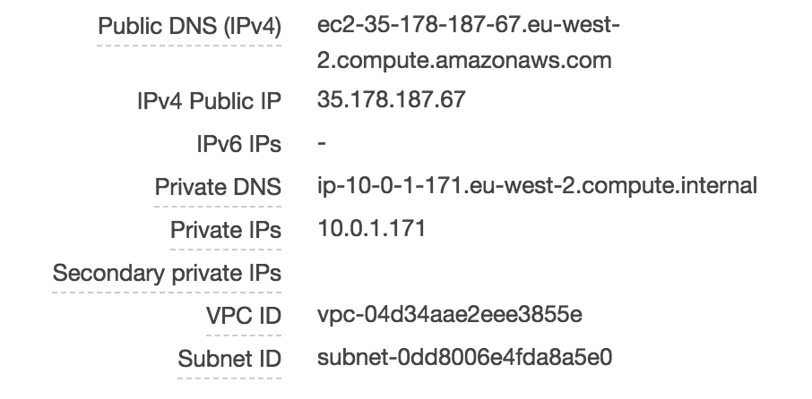
Let’s take a closer look at how public IPs work with EC2 instances. I have an instance running Amazon Linux - this instance has been assigned a public IP address of 35.178.187.67:
If I log on to my instance using SSH and execute an ‘ifconfig’ to view the IP addresses, it seems logical that we would see that public IP address listed in the output:
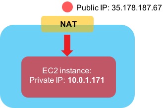
Hmm….we can see the private IP address here (10.0.1.171), but the public IP address is nowhere to be seen. How can that be? It turns out that AWS is doing Network Address Translation (NAT) behind the scenes. If traffic comes in from the Internet destined for the public IP address of your EC2 instance, AWS translates the destination address from the public IP to the private IP to allow it to reach the instance:
Alright, enough about IP addresses - time to look at how routing works in AWS networking.
Routing
In order to control how traffic flows in and out of the environments you create, every subnet is associated with a route table. A route table contains - believe it or not - one or more routes to control the flow of traffic. We’ve already seen earlier on that a default route (0.0.0.0/0) is often in place to direct traffic towards the Internet (via an Internet Gateway), but this isn’t the only type of route we can have. A route might point to a different type of gateway, such as a VPN gateway, a peering connection or VPC endpoint (we’ll look at these later).
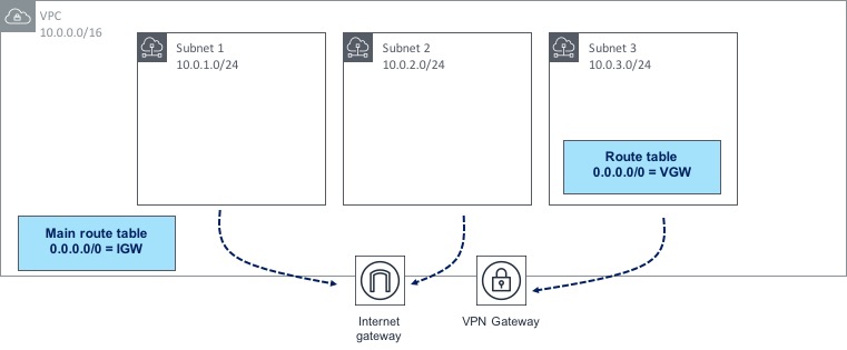
When you create a VPC, a special type of route table called the Main Route Table also gets created. If a subnet does not have an explicit association with a particular route table, then all routing for that subnet will be controlled by the main route table. However, it’s also possible to create a custom route table and assign that directly to your subnet(s) instead. Let’s look at a diagram to show how this works:
In the diagram above, we have three subnets within a VPC; two of those subnets are not explicitly associated with a route table, therefore they will use the main route table, which happens to have a route to the Internet through an IGW. Subnet 3 however has its own custom route table associated with it, which has a different 0.0.0.0/0 route towards a VPN gateway. By building and associating route tables in this way, you have a lot of control over how traffic is routed to and from your AWS environment.
NAT Gateways
Let’s say I have some EC2 instances sitting within a subnet. I don’t want those instances to be directly accessible from the Internet (i.e. no-one should be able to SSH in or send an HTTP request to any of my instances). However, I do need those instances to be able to connect out to the Internet so they can pick up patches, updates and so on. This presents a problem - if I give each of my instances a public IP address, that means they can connect out to the Internet (great), but it also means that someone from the outside could easily connect in to my instances (not so great).
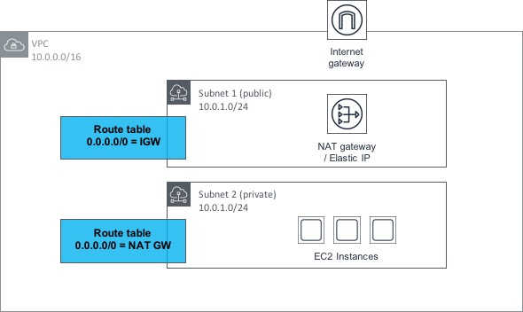
Fortunately, this problem is solved by a feature of AWS networking called NAT Gateways (or Network Address Translation Gateways). The idea behind a NAT Gateway is that it allows EC2 instances within a private subnet (i.e. one that does not have a route to an IGW) to access the Internet through the gateway, but it does not allow hosts on the Internet to connect inbound into those instances. As ever, a diagram will help to explain how this works:
OK, let’s step through this bit by bit. Within the VPC shown above, we have two subnets; one is public (i.e. it has a route to an Internet GW or IGW) and the other is private (it has no such route to an IGW). The private subnet has a number of EC2 instances contained within, all of which need outbound access to the Internet.
The public subnet has a NAT Gateway provisioned within it - this NAT Gateway also has an Elastic IP address associated with it. We discussed Elastic IPs earlier in the post - there is no real difference here, apart from the fact that the EIP is associated with the NAT Gateway rather than an EC2 instance. As the public subnet (in which the NAT Gateway resides) has a route to the IGW, the NAT Gateway can therefore reach the Internet.
Now, if we look at the private subnet, we can see that it has a route table associated with it that contains a default (0.0.0.0/0) route towards the NAT Gateway in the public subnet. This means that if the EC2 instances make a request outbound to the Internet, the request gets routed through the NAT Gateway and out to the Internet through the public subnet. However, there is no possible method for connections to be made inbound from the Internet to the EC2 instances.
Load Balancing
Load balancing is nothing new - it’s been around for many years in many types of environment. Load balancing gives you the ability to distribute traffic across similarly configured instances or other types of service. If for example, you have a web server farm consisting of a number of virtual machines / instances, load balancing will allow you to distribute traffic across these instances in a relatively even manner. Load balancing also allows you to make more intelligent decisions about where to send that traffic (for example, the failure of a single instance should mean that instance is removed from the farm of machines that the load balancer is sending traffic to, typically based on some kind of ‘health check’ functionality).
In AWS, there are few different types of load balancer available, as follows:
Classic Load Balancer: This is the original load balancer available from AWS - it is now considered a ‘previous generation’ load balancer and although it is still in widespread use, users should be encouraged to use one of the new generation load balancers (see below) instead.
Network Load Balancer: The NLB functions at layer 4 of the Open Systems Interconnection (OSI) model. This means that it load balances traffic based primarily on information at the TCP layer - although as of January 2019, it does now also support SSL / TLS termination.
Application Load Balancer: The ALB works at layer 7 of the OSI model (or the application layer). This means that it can be used for more advanced functionality, such as SSL / TLS termination, host or path based routing as well as support for multiple applications running on the same EC2 instance.
As the Classic load balancer is now considered ‘legacy’, I’ll focus on the NLB / ALB here. Have a look at this simple example:
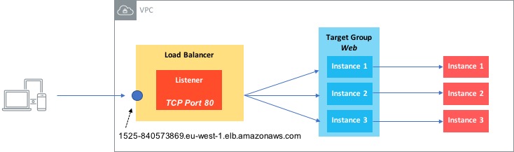
In this diagram, we have a Network Load Balancer (i.e. one that operates at layer 4). There are a couple of components involved with setting up a load balancer:
A Listener - this is essentially a rule that says ‘look at connection requests from clients on this specific port’. This rule then says ‘forward this request to one or more target groups’.
Target Group - the target group is a list of targets, such as EC2 instances or IP addresses that the requests will be forwarded to.
So in our example, we have a listener set up to look at requests on TCP port 80 and then forward those requests to a target group called Web, which contains three instances. As long the three instances are healthy, requests will be forwarded to them.
Note that the concept of listeners and target groups is common to both NLBs and ALBs.
One other thing to also mention is that load balancers can operate as either internal or Internet facing - load balancers that are designated as internal are for use by other hosts and devices within an AWS VPC and will not be accessible by clients on the Internet.
Finally, load balancers are availability zone (AZ) aware, so instances can be distributed across AZs and the load balancer will deliver traffic to them.
Security Groups
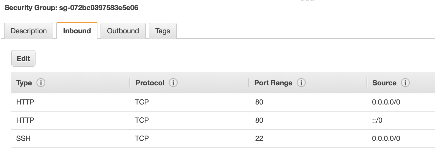
How do we secure access to and from the resources that we provision in AWS? Security Groups are used to lock down access into and out of your instances. A security group is essentially an access control list containing a set of rules that dictates which ports, protocols and IP ranges are allowed through to your resources. Here’s an example:
In this simple example, I’ve configured the security group to allow HTTP and SSH access from any source (0.0.0.0/0). In reality, you would ideally lock this down to specific IP addresses rather than allowing SSH from the entire Internet, but you get the idea.
One important point about security groups is that they are stateful. To understand what that means, think about an entry in a security group that allows traffic outbound from an EC2 instance. What about the return traffic back to that instance - is that allowed or denied? Because the security group is stateful, it automatically allows the return traffic back in - you don’t have to configure an entry yourself to allow that traffic.
VPC Peering
OK, so you’ve deployed a couple of VPCs - perhaps you have a different application deployed into each one, or maybe you have just split the app up and deployed it across multiple VPCs for more control. Now though, you’ve realised that actually there does need to be some communication between the VPCs you’ve deployed. Can it be done? Maybe you’ll have to route traffic from one VPC out to the Internet and back in to the other VPC? Well, that’s not going to be necessary, because there is a simple way to do this - VPC Peering.
VPC peering does exactly what you’d expect it to do - it allows you to peer two VPCs together in order for traffic to flow between them. The two VPCs could both be in the same AWS account, or they could be in two different accounts. You can even peer VPCs that reside in different AWS regions.
In order for VPC Peering to work, there are two main things you need to do:
Set up the peering connection itself
Set up routes that point to the ‘opposite’ VPC via the peering connection.
Here’s an example:
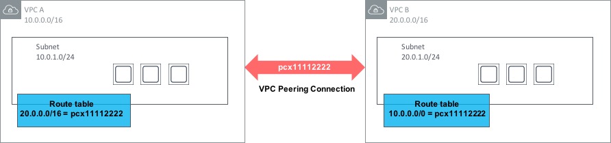
In the above diagram, a VPC Peering connection has been set up between VPC A and VPC B. VPC Peerings are always named pcx- followed by a number, so in this case our connection is called pcx-11112222. In order to set this connection up, one side creates a request. To activate the VPC Peering, the request must be accepted by the other side (i.e. the owner of the other VPC). But just having the peering in place doesn’t mean traffic will flow between the VPCs. To allow communication, a route is needed within each VPC that points to the address range of the opposite VPC and routes via the pcx-xxxxxxxx connection.
There are a couple of restrictions to be aware of with VPC Peerings. Firstly, it won’t work if you have overlapping CIDR ranges within the VPCs. So for example, if both VPCs you wish to connect have a CIDR range of 172.168.0.0/16, the peering won’t work.
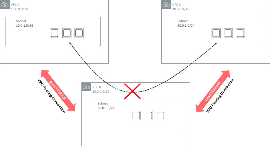
The second restriction on VPC Peerings is that they are non-transitive. What does that mean? Let’s say you have three VPCs - A, B and C. VPCs A and B are peered together, as are VPCs B and C. You might think that you will be able to communicate between hosts in VPC A and C - through VPC B - but this is not the case:
There are some ways around this - the Transit VPC design has been around for some time and uses a 3rd party network appliance (such as a Cisco CSR router running in the cloud) to provide ‘hub and spoke’ type routing between multiple VPCs. This design does have a few limitations however (such as limited bandwidth compared to VPC Peering), so this design pattern is likely to be superseded in many cases by a feature called Transit Gateway, which was announced at re:Invent 2018. Transit Gateway is a major step forward in the area of VPC connectivity, so let’s take a look at how it works.
Transit Gateway
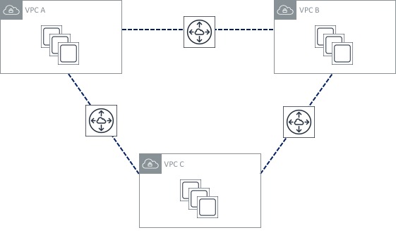
Let’s start by looking at an environment with three VPCs. Each of those VPCs is used for a specific function, but there is also a requirement to provide ‘any to any’ connectivity between the three VPCs. We can use VPC peering to achieve this - the resulting topology would look something like this:
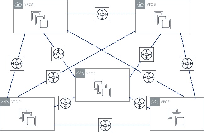
Not too bad, right? Three VPC peering connections isn’t too much to manage. Now though, I’ve decided to add two more VPCs to my environment. What does my peering topology look like now?
Oh dear! The number of peerings I have has increased significantly, which looks much more difficult to manage. Obviously this problem is going to get worse as I add more VPCs to my environment. The other issue here is that it becomes difficult to scale - there are limits on resources such as VPC peerings and routes that will probably prevent me from scaling this environment significantly. Previously, I could get around this by using the “transit VPC” design I mentioned in the section above, but that has its own limitations and drawbacks.
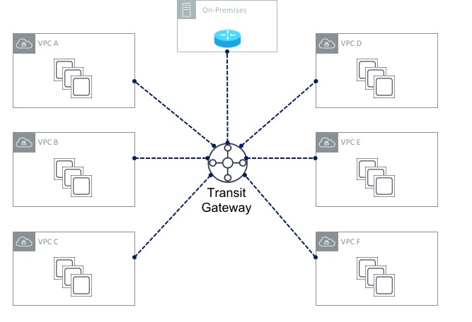
Transit Gateway solves this issue by creating a central point of attachment for VPCs and on-premises data centres via VPN or (later on) Direct Connect. With Transit Gateway in place, my topology now looks like this:
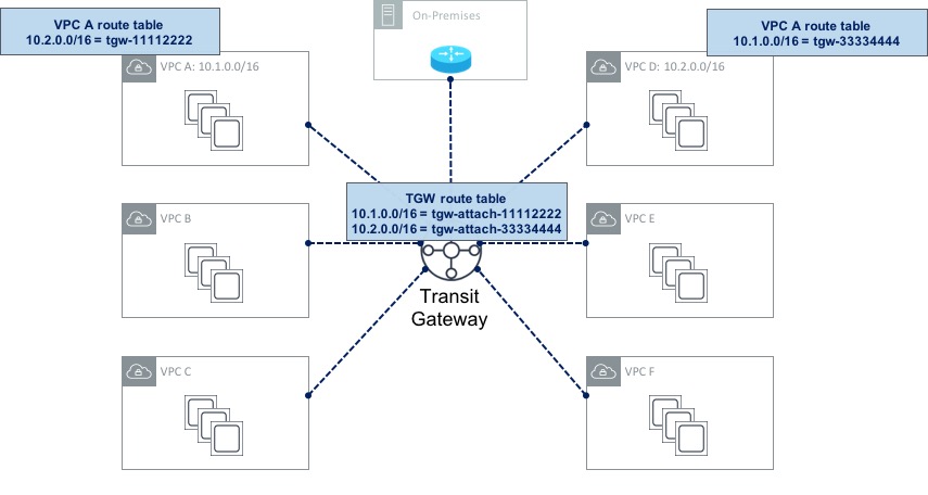
The Transit Gateway (or TGW for short) essentially acts like a large router to which your VPCs can all attach. The first thing you need to do is create the TGW itself. Once that’s done, you create Transit Gateway Attachments - each attachment connects a VPC to the TGW. By default, routing information will be propagated from each of the VPCs into the TGW routing table. This means that the TGW will have the information needed to reach the VPCs. However the reverse is not true - so each VPC needs to have routing information populated manually. For example, let’s say VPC A uses a CIDR range of 10.1.0.0/16 and VPC B uses a CIDR range of 10.2.0.0/16 as shown here:
In this example, the TGW route table has routes for both VPC A and VPC B (it may also have routes for the rest of the VPCs, but I’ve not shown those to save space). These routes have been propagated (i.e. they didn’t have to be configured manually). Now if you look at the route table for VPC A, you can see that it has a route pointing to VPC B via the TGW. This route had to be configured manually (it was not propagated). The same goes for VPC B.
Also shown in the above diagrams is a connection to an on-premises data centre. Before Transit Gateway was available, configuring VPN connections in a multi-VPC setup was sometimes difficult - it was necessary to configure a VPN Gateway (VGW) for each of the VPCs you had in place. With a Transit Gateway, you can configure a single VPN connection from the TGW to your on-premises data centre which can be shared by each of the attached VPCs. You can even configure multiple VPN connections from the TGW and traffic will be distributed over them to provide higher bandwidth (using equal cost multi-pathing).
Finally, it’s also possible to configure multiple route tables on a Transit Gateway in order to provide a level of separation in the network. This is very similar to the VRF (Virtual Routing & Forwarding) capability that most traditional routers have. As an example, you could connect each of the six VPCs shown above to a single TGW, but specify that VPCs A and B used the first route table (thereby allowing connectivity between them), while the rest of the VPCs use a completely separate route table. VPCs A and B would essentially be in their own network environment, while VPCs C, D, E and F would reside in a completely independent, isolated network with no connectivity to VPCs A and B.
PrivateLink & VPC Endpoints
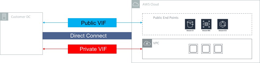
Think about a regular VPC with some EC2 instances residing within. Then imagine that those EC2 instances require connectivity to one or more AWS services (CloudWatch, SNS, etc) - for example, the EC2 instance might need to download some files from S3. What path does that traffic take? Under normal circumstances, that traffic will take the path over the public Internet; remember, S3, CloudWatch and other services are public services, which means that they are accessible via the Internet, or Direct Connect public VIF, etc.
This however might be a problem for some organisations - having their traffic leave the AWS network and on to the public Internet might not be all that appealing for some security conscious customers. VPC Endpoints and PrivateLink are designed to alleviate these concerns by allowing users to create private connections between their VPCs and AWS services, without the need for Internet Gateways, NAT and so on.
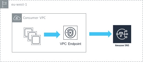
Here’s how it works.
In the above example, we have a single VPC containing a number of EC2 instances. Those instances want to access the AWS SNS service privately (i.e. not via the Internet). To achieve this, we create an interface endpoint inside our VPC that points towards the SNS service. What this actually does is creates a network interface (ENI) inside our VPC with a private IP address. That means that our EC2 instances are able to access the SNS service using the private IP inside the VPC, which results in the traffic never leaving the AWS network. You also have the option of creating an ENI in multiple subnets / availability zones for high availability.
One thing to be aware of is that there are a couple of services - S3 and Dynamo DB - that work in a slightly different way. These services use something called gateway endpoints - instead of creating an ENI inside the ‘consumer’ VPC, a gateway endpoint provides a target that you can route to. So in this case, you need to add a route to your routing table to S3 via the gateway endpoint.
VPC endpoints are a great feature, but there’s even better news - it’s also possible to create endpoints that point to your own services - i.e, not just the AWS services that we all know and love. Let’s look at an example.
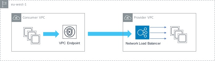
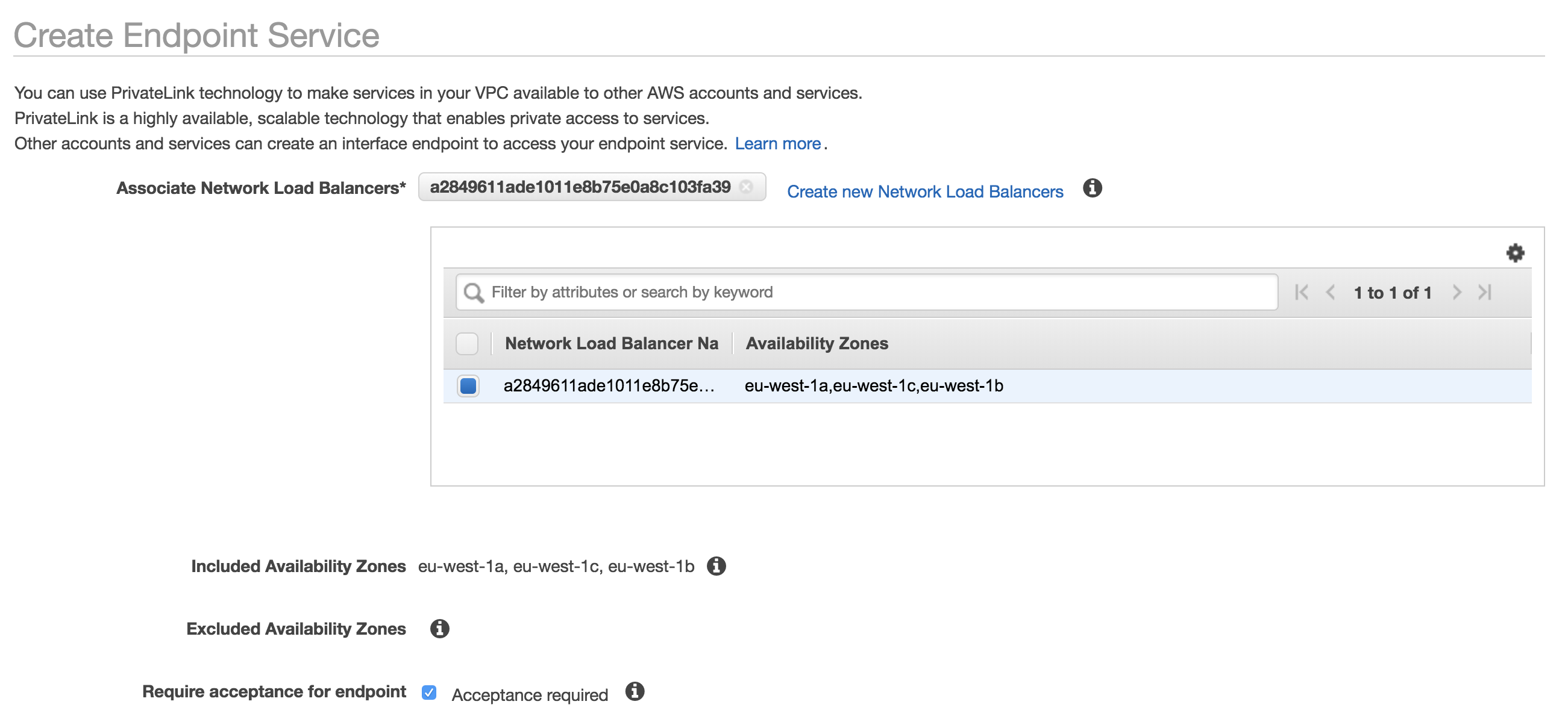
Here, we have two VPCs - one acts as the ‘consumer’ (i.e. it contains instances that will connect to the service) and the other is the ‘provider’ (it contains the service that we want to give our consumers access to. In order to set this up, we first need to configure a Network Load Balancer in front of our service in the provider VPC. This will load balance traffic across the instances that make up our service. Now that we have that in place, the next thing to do is to create an Endpoint Service. The Endpoint Service makes your service available to other VPCs through an endpoint.
Finally, we create an endpoint (similar to what we did in the AWS service use case) that points to the Endpoint Service that we just created. This enables private communication between the instances in the consumer VPC and the service that sits in the provider VPC.
Some might ask at this point: why not just enable VPC peering between the two VPCs? That would certainly be an option - the difference is that VPC peering enables full network connectivity between the two VPCs, while VPC Endpoints enable connectivity between services. In other words, with VPC peering, you are enabling fairly broad access, while with Endpoints you are allowing only specific connectivity between the services that you want.
Direct Connect
The ‘default’ method of connectivity into the AWS cloud environment is the Internet. This works just fine for many people, but equally, there are organisations who need to be sure that traffic to and from AWS is ‘private’ (i.e. not traversing the Internet). To satisfy this requirement, there are two main options: VPN connectivity (covered later in this post) and AWS Direct Connect.
Direct Connect is a private, dedicated line between AWS and a customer’s on-premises environment - Direct Connect provides a high bandwidth connection with predictable latency. 1Gbps and 10Gbps options are available, with lower connection speeds (50Mbps, 100Mbps, etc) available from AWS partners offering Direct Connect services.
A customer connects to AWS via Direct Connect at one of the available locations (more details here). It’s also possible to extend connectivity from a Direct Connection location to a customer’s location - this can be done with the help of an AWS partner.
Resources that you access inside AWS can generally fall into two categories; those resources that live inside a VPC (e.g. EC2 instances) and those that sit outside a VPC (S3, for example). Direct Connect can be used to provide connectivity to both types of resource, but it does need to be configured to do so. This is achieved through the use of virtual interfaces, or VIFs:
As you can see in the diagram above, a private VIF should be configured for connectivity into a VPC, whereas a public VIF needs to be configured for connectivity into services with a public end point (such as S3, RDS, ECS, etc).
In order for traffic to flow across a Direct Connect circuit, the correct routing information needs to be present at both the AWS and customer ends. To achieve this, the Border Gateway Protocol (BGP) is used - BGP is a widely supported routing protocol on most customer routers. From the AWS end, VPC CIDR ranges and / or public IP prefixes are advertised using BGP to the customer’s router. From the customer end, customer routes (or a default route) can be advertised to AWS.
Virtual Private Network (VPN) Connections
The other option for providing ‘private’ connectivity between an on-premises environment and AWS is to use a Managed VPN Connection. A VPN connection allows the user to configure a private secure tunnel using IPSec, typically over the public Internet. VPN connections are limited to 1.25Gbps, so don’t provide the same level of performance as a Direct Connect circuit.
VPN connections use two main components for the configuration: a Virtual Private Gateway and a Customer Gateway. The Virtual Private Gateway (or VGW for short) is the termination point for the VPN connection within a VPC. A VGW has a BGP Autonomous System (AS) number associated with it - this can be an AWS assigned number, or a customer number that you choose. The Customer Gateway is a resource that represents the customer side of the VPN connection (e.g. the “on-premises” side). When you configure a Customer Gateway, you specify the IP address of the VPN router within the on-premises environment, as well as the AS number of the on-premises side if using dynamic routing.
VPN Redundancy
One thing to bear in mind when setting up VPN connections is that each connection uses two tunnels for redundancy purposes. This ensures that connectivity remains should an underlying issue affect one of the VGWs. However, having two tunnels doesn’t provide protection against the failure of the customer gateway (as both tunnels terminate on the same CG). To protect against the failure of a single Customer Gateway, it’s possible to set up a separate VPN connection and terminate this on a different CG at the on-premises end.
In the above diagram, there are four tunnels in total - two associated with the first Customer Gateway and another two associated with the second. In this scenario, if the first CG fails, the second is still available to handle the VPN connectivity to AWS.
OK, this has been a long post so I think I’ll stop there. Clearly there’s a lot to networking in AWS - hopefully this post has given you an idea of how things work. In the next post, we’ll dive into storage in AWS.